CFD

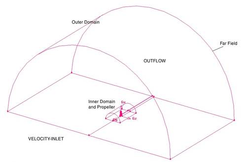
Figure 8 shows the standard computational domain created for CFD simulations.  It consists of two domains: an inner and outer domain.  The inner domain is the smaller of the two half-cylinders, in which the propeller blade and cone are located (figure 9).  The outer domain is the bigger of the two half-cylinders and completely encompasses the inner domain.  The inner and outer domains were assigned the radius of 150mm (approximately 2 blade lengths) and 1600mm (approximately 29 blade lengths), respectively.   

Figure 8:  3-D computational domains

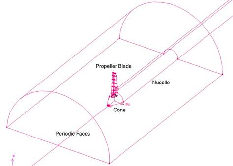
Figure 9:  Inner domain

The inlet boundary was placed 18 blade lengths in front of the blade and the outlet was placed 18 blade lengths behind the blade. Due to the rotating reference frame, a far-field boundary was established at a constant radius of approximately 29 blade lengths from the blade. These boundary conditions were placed far from the propeller in order to reduce interaction with the flow induced by the propeller and simulate and open air environment. The nosecone of the motor and nacelle (figure 11) were also constructed as part of the CFD model in order to mimic the setup of wind tunnel testing. The nacelle was extended to the outlet in order to simplify the geometry and CFD boundary conditions.

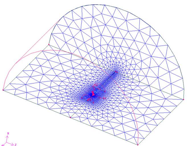
Figure 10: Mesh of the CFD model

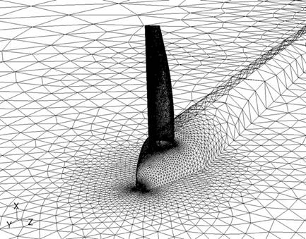
Figure 11:  Isometric view of blade, cone, nacelle, and inner periodic faces

The inlet and far-field zones were assigned as velocity inlet boundary conditions which Fluent describes as a zone where “the total (or stagnation) properties of the flow are not fixed, so they will rise to whatever value is necessary to provide the prescribed velocity bistrubution.”¹³ The outlet was assigned an outflow boundary condition, which Fluent says “are used to model flow exits where the details of the flow velocity and pressure are not known prior to solution of the flow problem.”¹³ In other words, no parameters are specified at outflow boundaries; FLUENT extrapolates the required information from the interior. The no-slip boundary condition was used for all walls and the Periodic rotational boundary condition is used for the two horizontal periodic planes.

It can be seen in figure 10 and 11 that the mesh spacing is smaller within the inner domain and coarser in the outer domain.  It was desirable to obtain this kind of packed (clustered) mesh in the vicinity of the propeller blade, so that FLUENT (solver) will be able to resolve the wall boundary layer and tip vortices.  The purpose of having the two domains is to simplify this meshing process and to localize the finer mesh within complicated flow regions.

In order to achieve a mesh-independent solution, it is necessary to perform a mesh refinement to increase the number of cells and re-simulate.  The boundary layer was specially chosen for mesh refinement because the flow is in the region of high velocity gradients. Initially, four boundary layers were applied, and it was increased by one or two layers in each mesh refinement.  For example, straight blade was simulated with 4 (figure 12), 6, 7 and 8 (figure 13) boundary layers at the same free stream velocity.  Percentage change in the efficiency between each increased boundary layer simulation was calculated to be 15.4%, 0.76% and 0.016%. In all simulations second order discretization scheme is used for the momentum.

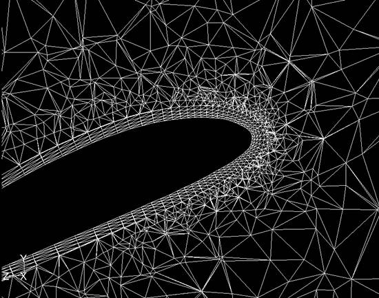
Figure 12: Projection of 3-D mesh onto the cross sectional plane

(4 boundary layers)

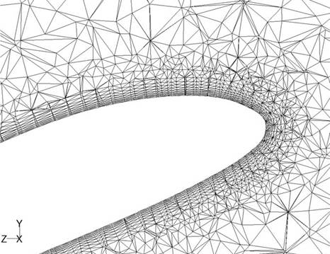
Figure 13: Projection of 3-D mesh onto the cross sectional plane

(8 boundary layers)